An Algorithm for Affordable Vision-Based GNSS-Denied Strapdown Celestial Navigation

adminJanuary 20, 2025

0 0 10 minutes read

A modular celestial navigation system should be mounted rigidly with respect to the AHRS. The orientation of the aircraft, $C_{l / b}$ , is provided by the autopilot. The orientation of the camera, $C_{b / c}$ , is unknown and must be calibrated to obtain accurate positional information. For the purposes of this study, we assume that the precise orientation of the camera remains unknown, and we consequently accept that the individual position estimates will be erroneous. It will be shown later that this misalignment may be overcome through the use of averaging. This is particularly useful given that the camera itself may be mounted separately from the autopilot, thus being subjected to factors such as vibration, aerodynamic loading, or changes in AHRS biases, which cause the relative orientation between the AHRS and the camera to change over time.

3.1. Star Detection and Tracking

Stars are detected within an image using a basic binary thresholding operation. Given a mean pixel value within the frame,

μ

, and standard deviation,

σ

, a binary threshold is set at

μ + 5 σ

, as advised in [17]. The contours are extracted, and an agglomerative clustering algorithm is applied to cluster redundant detections.

Once detected, a standard Kalman filter is used to track individual stars between frames. Each star is defined by its state vector:
and a constant sized bounding box. The states

u, v, \dot{u}, and \dot{v}

describe the x position, y position, x velocity, and y velocity of the star on the image plane, respectively. The position of the star is taken to be the subpixel maxima, computed as a weighted average of the

3 \times 3

Region of Interest (ROI) centered on the peak pixel value, as described by [18]

$(u, v) = (\frac{\sum_{i, j} I_{i, j} u_{i}}{\sum_{i, j} I_{i, j}}, \frac{\sum_{i, j} I_{i, j} v_{j}}{\sum_{i, j} I_{i, j}})$

(12)

The state transition matrix

F

is defined assuming a constant velocity as follows:

$F = [\begin{matrix} 1 & 0 & Δ t & 0 \\ 0 & 1 & 0 & Δ t \\ 0 & 0 & 1 & 0 \\ 0 & 0 & 0 & 1 \end{matrix}]$

(13)

The position and velocity of the stars are observed directly; therefore, the observation matrix

H

is defined as the

4 \times 4

identity, such that the observation equation is simply given by

Following the standard Kalman filter equations, the a priori state and covariance estimates are computed:

${\hat{P}}_{k + 1} = F P_{k} F^{T} + Q$

(16)

for the covariance matrix $P_{k}$ with process noise $Q$ . The innovation is calculated as follows:

$y_{k} = z_{k} - {\hat{x}}_{k + 1}$

(17)

with covariance, $S_{k}$ , given by

$S_{k} = {\hat{P}}_{k + 1} + R_{k}$

(18)

where $R_{k}$ is the measurement noise. The Kalman gain is computed as follows:

$K_{k} = {\hat{P}}_{k + 1} S_{k}^{- 1}$

(19)

and the posterior updates are applied to the a priori estimates:

$x_{k + 1} = {\hat{x}}_{k + 1} + K_{k} y_{k}$

(20)

$P_{k + 1} = (I - K_{k}) {\hat{P}}_{k + 1}$

(21)

The measurement noise,

R_{k}

, is defined as a diagonal matrix, with elements equal to

[0.5 0.5 1.0 1.0]

, and the process noise is also defined as a diagonal matrix, with elements equal to

[4.0 4.0 2.0 2.0]

. The measurement noise was selected based on the calibration accuracy of the camera, and the process noise was experimentally tuned to minimize the occurrence of lost tracks under high motion conditions. The a priori state estimate is used to propagate the bounding box containing the region of interest, within which the peak is detected using Equation (12). The bounding box is centered on

[u, v]

, rounded to the nearest pixel. The width and height of the bounding box were fixed at 21 pixels for this imaging system, given an image resolution of

1936 \times 1216

and a field of view of 53.5 deg. A visual snapshot of the tracking system can be seen in Figure 2.

3.3. Position Estimation

The star tracker in Section 3.1 operates on distorted images. The pixel location from each star tracker is extracted. rectified, and subsequently converted to a unit vector in NED coordinates according to Section 2.1. Given an observation

X^{l} = {[x y z]}^{T}

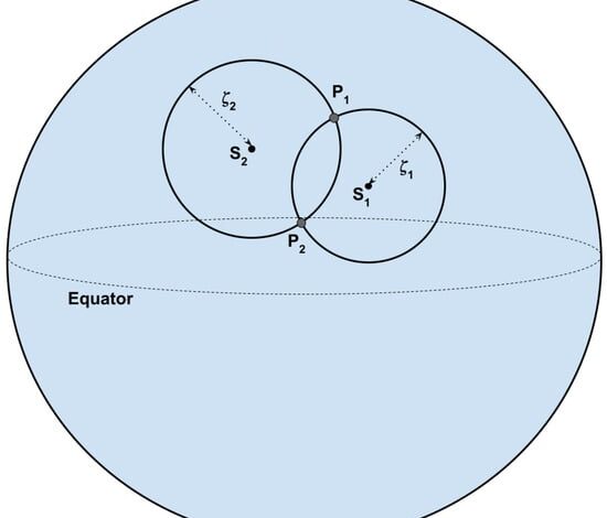
, the elevation of a star above the horizon is calculated as

$e l = - {tan}^{- 1} \frac{y}{\sqrt{x^{2} + y^{2}}}$

(22)

and, subsequently, the zenith-angle $ζ$ is calculated as $90 - e l$ .

In the initial case, the camera orientation $C_{l / b}$ is not known to a high level of precision. Assuming that an attempt is made to mount the camera in alignment with the autopilot, an initial DCM may be formulated from some combination of 90° Euler rotations. It will be seen that as long as this orientation is accurate to within a hemisphere of tolerance, the exact value does not matter, as it will be recalculated in flight.

If a minimum of six stars are visible within the frame, a Random Sample Consensus (RANSAC) approach to position estimation may be used to remove bias from false detections. RANSAC is a technique used to identify outliers in sample data and omit them from the estimation process. This is useful for detecting misidentified stars or for removing non-star detections (such as satellites or overhead planes). In the context of position estimation, the RANSAC algorithm randomly selects three stars to generate a position estimate. Subsequently, the algorithm compares the location of the remaining stars against the position estimate. If the remaining stars are within some heuristic tolerance, they are considered inliers. If they are outside of tolerance, they are considered outliers. The position estimate which minimizes the mean squared error of the inliers is chosen as the estimate. A pseudocode implementation of this RANSAC position estimation is outlined in Algorithm 1.

Algorithm 1 Position-RANSAC

$C_{l / b}, C_{b / c}$

$G H A Γ \leftarrow g e t G H A A r i e s ()$

$A s \leftarrow []$

$P s \leftarrow []$

for $o b s$ in $o b s e r v a t i o n s$ do

$a z, e l = c o m p u t e A z E l (o b s, C_{l / b}, C_{b / c})$

$a, b, c, p = c o m p u t e P o s i t i o n C o e f f i c i e n t s (G H A Γ, a z, e l, o b s . r a, o b s . d e c)$

$A s . a p p e n d ([a, b, c])$

$P s . a p p e n d ([p])$

end for

$i n l i e r s \leftarrow 0$

$o u t l i e r s \leftarrow 0$

$b e s t e r r o r \leftarrow inf$

$x \leftarrow [0, 0, 0]$

for
$0 < i < i t e r a t i o n s$
do

$j \leftarrow$ 3 randomly selected indexes

build $A$ and $p$ using $A s [j]$ and $P s [j]$

$\hat{x} \leftarrow {(A^{T} A)}^{- 1} A^{T} p$

$i n l i e r e r r o r \leftarrow 0$

for all remaining indexes k do

$E \leftarrow P s [k] - A s [k] \hat{x}$

if $E < t o l e r a n c e$ then

$i n l i e r s$ += 1

$i n l i e r e r r o r$ += $E$

else

$o u t l i e r s$ += 1

end if

end for

if $i n l i e r s : o u t l i e r s > a c c e p t a b l e r a t i o$ then

$m e a n e r r o r = i n l i e r e r r o r / i n l i e r s$

if $m e a n e r r o r < b e s t e r r o r$ then

$b e s t e r r o r = m e a n e r r o r$

$x \leftarrow \hat{x}$

end if

end for

$ϕ \leftarrow {tan}^{- 1} (\frac{x [2]}{\sqrt{x {[0]}^{2} + x {[1]}^{2}}})$

$λ \leftarrow {tan}^{- 1} (\frac{x [1]}{x [0]})$

return
$ϕ, λ$

We first demonstrate that, in the general case, the DCM

C_{l / b}

is not fixed during flight. In an integrated solution, the celestial system would provide attitude measurements to the EKF, and the offset from this attitude would be estimated. As a modular solution, however, this is infeasible. Taking the output from the EKF to be the true orientation of the aircraft, we can use the true GPS position to compute

C_{l / b}

. We use the Kabsch-RANSAC methodology presented in [19] to calculate the ideal rotation between a star’s theoretical location and its actual location. In conjunction with the autopilot output, this rotation yields

C_{l / b}

. Testing over an 89 s section of flat and level flight, it can be seen in Figure 5 that the camera roll angle shifts by approximately 0.2°, the pitch angle shifts by approximately 0.05°, and the yaw angle shifts by approximately 0.3°. In the context of celestial navigation, these are significant perturbances which, had the offsets been attributed to position as opposed to camera orientation, would have been interpreted as around 30 km of positional offset. Indeed, by assuming that

C_{l / b}

is fixed, we can see in Figure 6 that the latitude drifts by approximately 0.2° over the same short window of flat and level flight. Over an extended period (hours), the orientation may shift such that positional errors are in the range of hundreds of kilometers.

It is clear that a stand-alone celestial module cannot function in the conventional manner with consumer-grade hardware, unless the autopilot is capable of integrating the attitude output from the celestial system into its own filter and estimating the camera orientation. We will demonstrate now a method which, given a very rough initial estimate of the camera orientation, is capable of returning position estimates to within 4 km. This is significant in the context of long flights, where alternative dead-reckoning solutions would experience positional drift that is either linear (assuming velocity measurements are available) or quadratic (assuming only acceleration measurements) as a function of time.

By performing a rotation through 360° of compass heading, at an approximately constant yaw rate, the position estimates can be averaged to find an approximation of the orbital center. Provided n images throughout an orbit are available, there exists n latitude and longitude estimates, which may be expressed as unit vectors in the Earth Centred Earth Fixed (ECEF) frame

p_{i}^{e c e f}

. The mean position is taken to be the mean of these vectors:

${\bar{p}}^{e c e f} = \frac{1}{n} \sum_{i = 1}^{n} p_{i}^{e c e f}$

(23)

The latitude and longitude are simply calculated as

$ϕ = {sin}^{- 1} (z)$

(24)

where x, y, and z are the elements of the mean position vector.

Once an initial position estimate has been formulated, it may be used to calculate a more precise estimate of the camera orientation

C_{b / l}

. The aim of orientation estimation is to find the rotation matrix

R

that minimizes the residual error between a set of observations

u^{c}

represented in the camera frame of reference and a set of theoretical unit vectors

v^{l}

in the NED frame of reference:

$E = \sum_{i = 1}^{n} ‖ v_{i}^{l} - R u_{i}^{c} ‖^{2},$

(26)

In this case, the rotation matrix

R

is composed of the aircraft DCM,

C_{l / b}

, and the camera DCM,

C_{b / c}

:
where we accept

C_{l / b}

as a deterministic output from the autopilot, and so the camera orientation may be found given

R

and

C_{l / b}

$C_{b / c} = C_{l / b}^{T} R$

(28)

Each observation

u_{i}^{c}

is correlated with a database star. This correlation is obtained through star identification. During the instantiation of the star tracker, a lost-in-space log-polar star identification algorithm is used to determine the IDs of each star in the frame [20]. The theoretical position vectors

v_{i}^{l}

in the NED coordinates are generated from the star’s right ascension and declination, the time of observation, and the estimated latitude and longitude [13]. This allows for the use of the Kabsch algorithm [21] to find the rotation

R

between the observed stars and the database stars. Following the implementation in [19], the algorithm is provided in Algorithm 2, where

A

is the matrix of n observation vectors with dimension

[n \times 3]

and

B

is the matrix of n theoretical vectors, also with dimension

[n \times 3]

. The resulting rotation

R

is used in conjunction with the most recent autopilot attitude data to find the camera orientation

C_{b / c}

Algorithm 2 Kabsch

Translate vectors in $A$ and $B$ such that centroid is at origin

Compute the matrix $C = A^{T} B$

Compute the singular value decomposition $U, Σ, V = SVD (C)$ such that $C = U Σ V^{T}$

Set diagonal elements $Σ_{1}$ through to $Σ_{n - 1}$ = 1.

if $det (UV) > 0$
then

$Σ_{n}$ = 1

else

$Σ_{n}$ = −1

end if

Compute the rotation matrix $R = V Σ U^{T}$

Once the camera orientation has been found, two options are presented, depending on the computational power of the flight computer. If the computer is capable of parallel processing, then the set of theoretical star locations

v^{l}

may be re-calculated using the updated latitude and longitude, and the estimated positions may be re-calculated using the updated camera DCM

C_{b / c}

. This enables the system to recursively converge on a position estimate from a single set of orbital data. Alternatively, it is possible to repeat an orbit and calculate a new set of latitudes and longitudes. This method does not require post hoc processing and may be better suited to real-time applications. For the purposes of this study, we use the former method, as this allows us to treat each orbit as an independent sample, yielding an independent position estimate, thus giving us deeper insight into how the characteristics of a given orbit affect the position estimate. An example of this process can be seen in Figure 7.

3.1. Star Detection and Tracking

3.3. Position Estimation

admin

Related Articles

Spotify is full of AI music

Fixing Recursions In Grammar – Siddharth Mishra

Show HN: Obsess Jobs – Apply to jobs in your sleep

Why HNSW is Not the Answer to Vector Databases

Leave a Reply